Simulation: Phased Arrays
Posted on May 8, 2025
How do you focus waves? One way is to use phased arrays. I recently became interested in phased arrays after watching this amazing video.
From what I understand, a phased array is basically a collection of regularly spaced oscillators that emit in the outward direction, each oscillator producing a wave with a spherical symmetry. The idea is that, due to interference, the array produces a (somewhat focused) beam of waves. The more oscillators, the more focused the beam becomes. These beams can be steered by subtle tuning of the phase difference between the individual oscillators. If all oscillators are oscillating in unison, the resulting beam will propagate perpendicular to the array.
This phenomenon is used for a range of tech applications, such as antenna’s (electromagnetic waves), and ultrasound imaging (ultrasonic acoustic waves). I was a bit inspired by this phenomenon, and formulated a vague goal for myself: to build a 2D phased array, for scanning 3D objects. The oscillators in question will be transducers that produce ultrasonic waves of 40 KHz, and should be individually controlled through a microcontroller. The amount of oscillators I have in mind is a 4x4 or 5x5 grid, the amount being limited by the amount of outputs on the microcontroller.
As a first step, I thought it would be a good idea to simulate these systems on a computer, to get a feeling for the behaviour of phased arrays. I started out with a script in Python that can simulate a 1D array of oscillators, it can be found here. Essentially, it’s just a superposition of circular waves,
\(// \psi(x,y)=e^{ikr}\),
for a spatial grid of 512 by 512 pixels.
I tried a row of 4 oscillators:
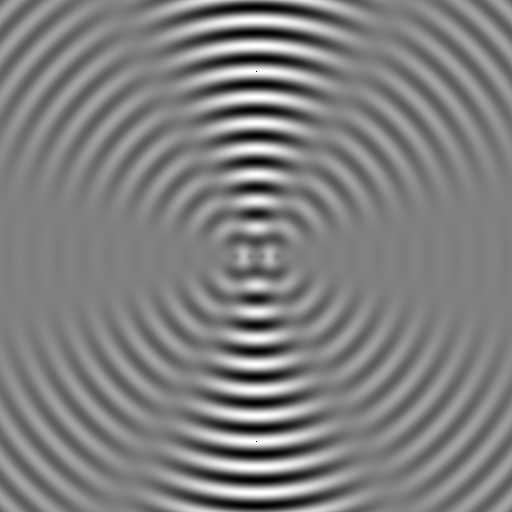
then steered it by changing the relative phases:
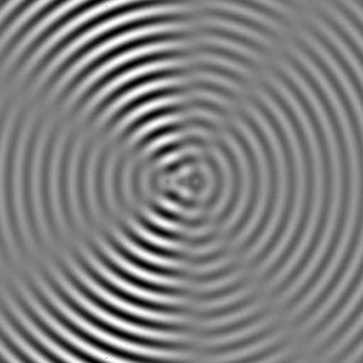
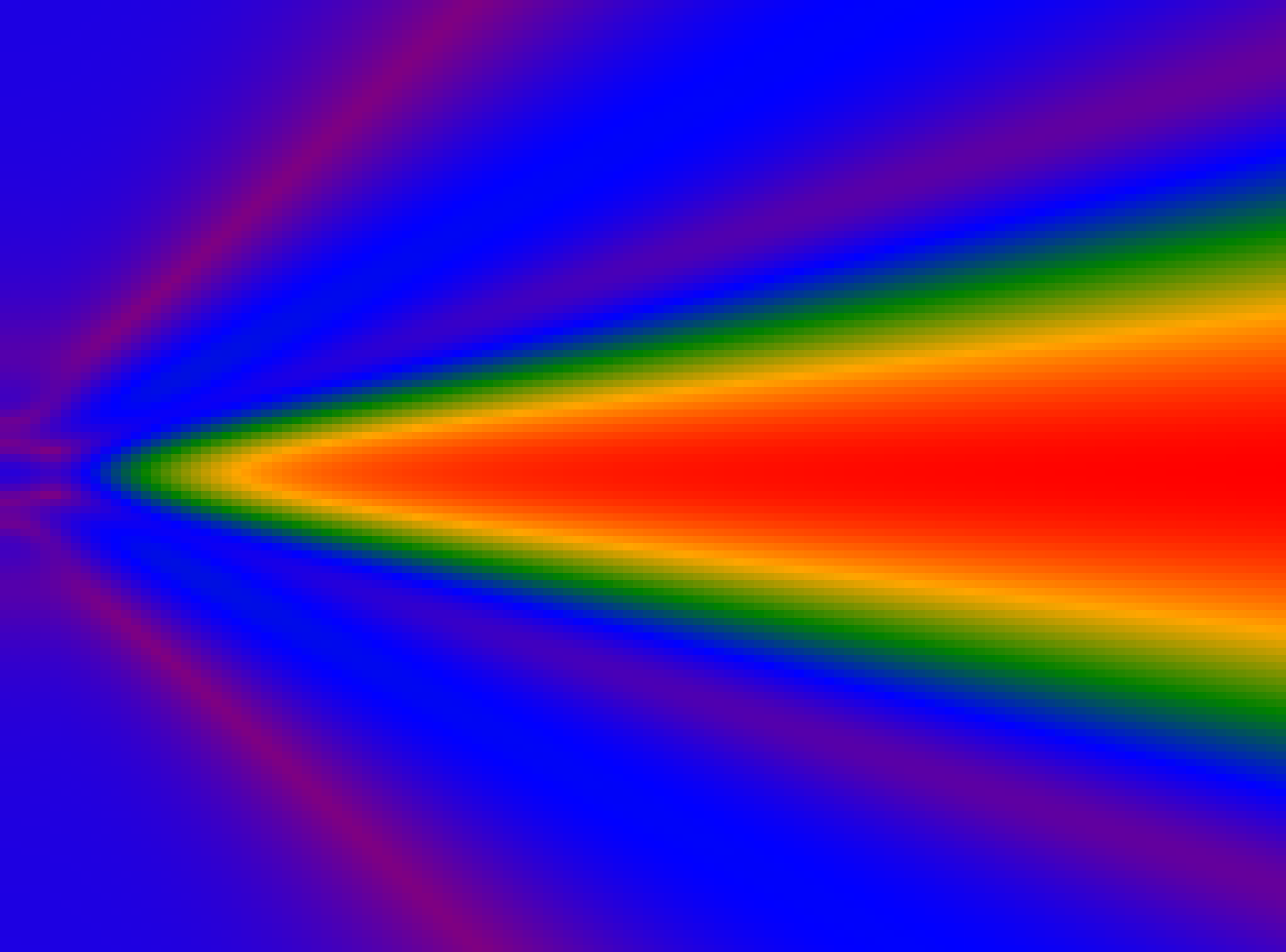
and extended it to 6 oscillators. It can be seen that the beam is more narrow:

and here is the power of the beam:
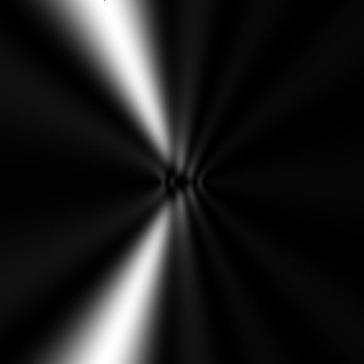
I did not take any attentuation of the waves into account, since I was just interested in the directionality.
Of course, I wanted to take it to the next level by extending these simulations to the third dimension, in order to investigate two dimensional arrays of oscillators. Since this is a bit heavy for Python (4 nested for-loops, need I say mo’), I turned to my favorite language, Julia. I wrote an object oriented script that treats the simulation like an object, and utilized the GPU for the heavy lifting, using the CUDA library. All of this was done in a handy Jupyter Notebook format. Just create a simulation using sim = SimulationWorld(…), and run it by run(sim), and the total psi(x,y,z) is outputted (is outputted a word?). This way, a grid of 512 x 512 x 1024 voxels (a quarter billion points), for 25 oscillators is simulated in 5 seconds on a laptop RTX 2060 graphics card.
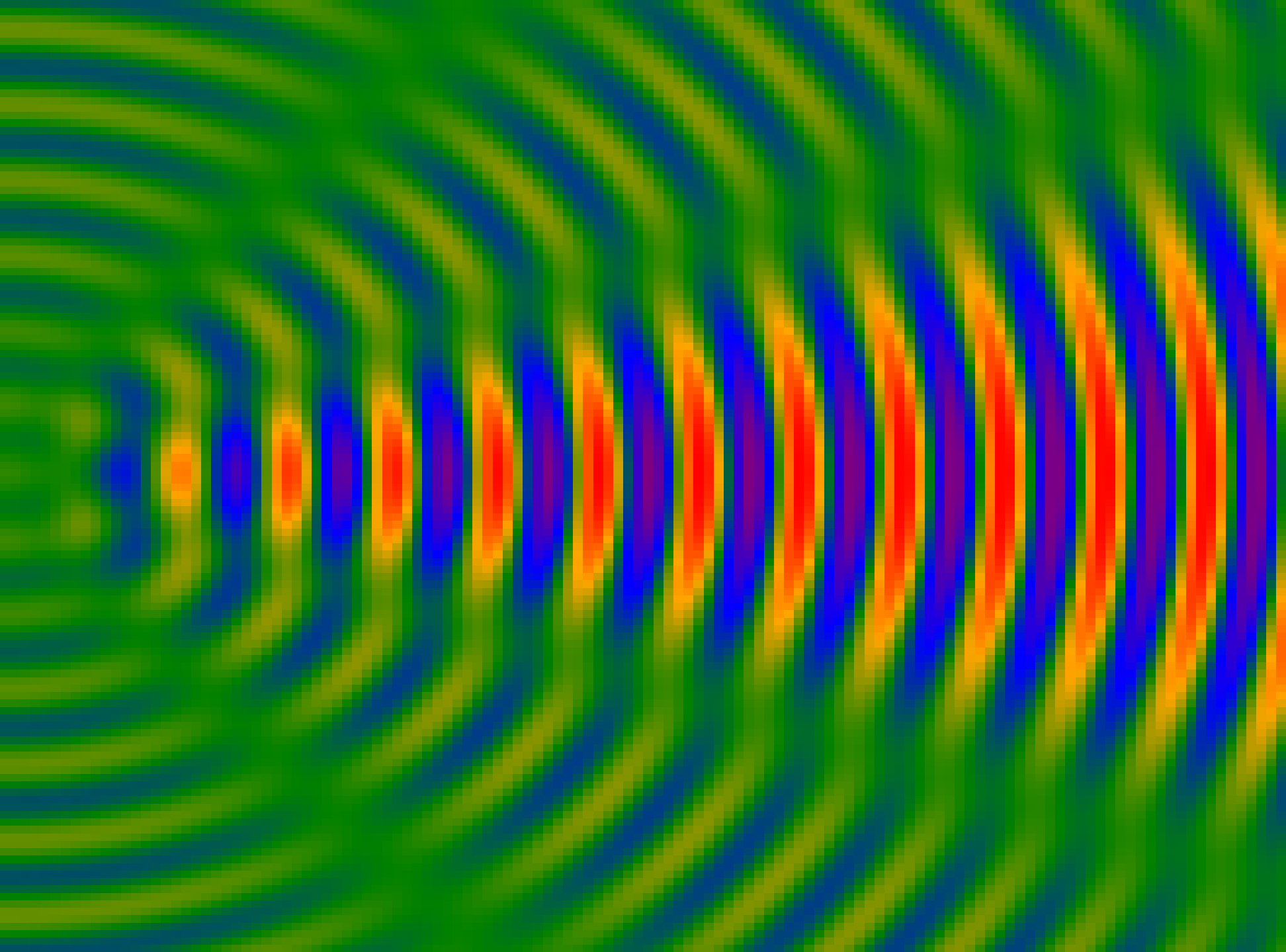
Let’s focus on a simulation of 25 oscillators, i.e. a 5 by 5 grid. The spacing between the oscillators is half a wavelength. We can then take slices through the middle of psi(x,y,z) block to inspect the beam (the emitters are on the left side):
We can also inspect the power of the beam over this slice:
The nice thing about full 3D instead of 2D simulations is, besides the increased accuracy, the possibility of 3D visualisation. Let’s make beautiful 3D images of the beam making its way through space. One way to do this is by 3D voxel plotting, but this will burn your graphics card for the size of grid that we are interested in. Instead, it would be good to wrap isosurfaces of equal pressure/amplitude around the different regions in space. For this, we first have to find a suitable threshold for the amplitude, both positive and negative, and group connected regions together. Then, we wrap isosurfaces around these regions using a marching cubes algorithm (it’s part of a Julia package), which results in meshes for both positive and negative regions. Now, we can save these meshes into .obj files, and import them in Blender. I have to admit that in this last section I relied quite heavily on ‘vibe coding’, but whatever works works, and the result is quite amazing.
Here are waves emitted from the 25 oscillators, with a oscillator spacing of 0.5 wavelengths:
It can be seen that this leads to a nice, focused cone, with only small lobes on the sides. What happens when we increase the distance between the oscillators to a full wavelength?
It can be seen that significant side lobes exist, that carry a large portion of the total energy. The main beam also lost it’s circular shape, and instead has a more square-like outline. This seems like a good platform for studying the behaviour of the phased array. The next step is the experimental realization of such an array, I hope this will turn out good too. Stay tuned people.