Here is how I made it:

WRITING THE SIMULATION BACKEND

First things first: what are we simulating? A flexible string. The string is modelled as a set of coupled masses, where the coupling occurs through (invisible) springs. The physics is then pretty simple, as for the two dimensional case, the force on each mass can be described by:

where i is the index of the particle in question, k is the spring constant in Hooke’s law, and r is the distance to the neighbour, where r_0 is the initial offset (note the extra r ̂ in comparison the 1D case). We can then integrate Newton’s law to find the position of each particle, at each point in time:

One of the finer ways to do this is to use a velocity-Verlet solver, which is a so called symplectic solver that conserves energy (in contrast to, for example, a simple Euler solver that tends to dissipate energy). I will not go into details on this algorithm, but it involves some separate steps to calculate velocity, Force (acceleration), and position.

And that is basically all there is to it, if you have enough of these masses, you effectively have a flexible string. How do we describe this to a computer?

The language of choice is C++, since it’s fast, and it is supported by Android Studio (a great program for making Android apps). C++ has gotten a bad reputation lately for it’s unsafety and verbose (at least modern versions are verbose) language, but I like the easy control of pointers and the possibility of having classes. If you don’t know what a class is: it’s a struct which also allows functions as members, and does an automatic type definition. The latter means that you can for example define a car as a type: class Car{..}; , and then instantiate this type like so: ’Car Skoda;’ , similar to ’int a;’. This is one of the cornerstones of object oriented programming, and I love it. Anyway, before we define a system of coupled masses, we can define a little 2D math library, not just out of necessity, but also because it’s fun and useful to learn (I see every programming project as a chance to learn C++).

MATH LIBRARY

Let’s define a class called Vec2, and outfit this class with functions (methods) to define normal operations like summation and multiplication, but for two dimensions. This is called operator overloading. I chose to do this in a separate header file, .h, and have the definition of the functions in a .cpp file. It looks then a bit like this (this example shows the definition of summation of 2D vectors in the .h file):

Vec2 operator+(const Vec2& other) const;

And here is the implementation in the .cpp file:

Vec2 Vec2::operator+(const Vec2& other) const {
    return Vec2(x + other.x, y + other.y);
}

Simple enough, add two Vec2’s and return a Vec2 with the sum! The & in this case means that you pass the variable directly by reference, i.e. there is no copying of variables. The const prefix is just a hint to the compiler, and makes things as fast as possible. I also needed some custom functions for stuff like absolute distance (the r in equation 1), the direction, and the dot-product. For example, the distance function is defined as:

float Vec2::DistanceTo(const Vec2& u) const{
	return std::sqrt((x - u.x) * (x - u.x) + (y - u.y) * (y - u.y));
}

Indeed you can recognize Pythagoras in there. Doing it this way, if you have two Vec2’s that indicate a position, since DistanceTo is a member function, you can evaluate the distance in this fun way:

position_1.DistanceTo(position_2). 

I did it the same for direction and dot product, direction_1.Dot(direction_2). The more normal case would be to define it such that you can write Dot(direction_1, direction_2), but in my way it has the order of normal maths, which I like.

And that was it for the math library! Now on to the particle system and simulation.

PARTICLE SYSTEM AND SIMULATION

Let’s start by defining a class, Particle, which has physics properties like position, velocity and acceleration, and mass. Additionally, it has Boolean properties like ‘fixed’ and ‘simulable’, the latter will come in handy when we will interact with the system, and the former is useful to fix a string at its ends. The wildest property it has, is a list of neighbours, which is a vector containing Particle’s. Indeed, the Particle class has a member of it’s own type! It is written as:

std::vector<Particle*> neighbours = std::vector<Particle*>();

The way of setting the array with std::vector is safer than using neighbours[]. The attentive reader will note that it is not really an array of particle data, but rather pointers to particles (note the * ). Indeed, this is useful because otherwise we store copies of the initially defined particles only, and the info of the particles will not be updated during the simulation. With pointers you make sure to just look up whatever is at that memory address.

After having defined our particle, we define a system of particles in a class:

class ParticleSystem;

This has one member only, which is an array of Particle’s. The constructor function of this class then creates the total simulatable string from two input variables; the amount of particles, and a cutoff distance:

ParticleSystem(const int N_Particles, const float r_cutoff){…}

This cutoff distance serves to determine which neighbours belong to a particle’s neighbour list, i.e. if the initial distance is smaller than the cutoff distance, it will be included in the neighbour list. This list is constant throughout the simulation, i.e. the amount of neighbours will not change. We will see later that the neighbour list allows for a flexible approach to the string: it makes also easily possible topologies other than of the trivial string. It is also worth noting that the neighbourlist essentially creates a linked list. For example, if you want to find the x-component of the position of the third neighbour to the left of particle i, you can find it like so:

particleSystem.particles[i].neighbours[1].neighbours[1].neighbours[1]->position.x; 

(If you wanted to go to the right, just replace 1 with 2 in the indexes). Yes -> we are dereferencing a pointer to get the position (remember the neighbour list is a list of pointers!). This may just seem like a fun little fact, but it adds a flexible way of including higher order interactions such as angle bending (whose emergent property is string stiffness).

SIMULATION

Having taken care of our particles, let’s define our simulation. As you have noticed, I like classes, so let’s set up a simulation class: class Simulator{};. In this class we include some properties like the spring constant and the tension in the string, and perhaps damping. The foremost members of this class are the functions that describe the solver, which integrates the equation of motion for a set timestep. Essentially, the velocity Verlet algorithm comes down to:

void verletSolver(ParticleSystem* ps) {
        updatePositions(ps, timeStep);
        updateForcesAndAccelerations(ps, springConstant, springDamping, stringTension);
        updateVelocities(ps, timeStep);
}

This updates the positions for one timestep delta t. This means that position is a mutable variable, and will be updated many times. Some people are opposed to using mutable variables, not in the least John Carmack, but honestly I would not know how to do this in another way for a simulation that is in principle infinitely long. I could initiate a very large array and write to that, but at some point it will be full and the party is over. The gist of this solver is in our updateForcesAndAcceleration; function. Wtf? Indeed, it just calculates the force looping over all the particles, and the neighbours, so that means two nested for loops, a big one and a small one. In order to calculate the force, you also need to know r0, the offset, see eq 1. This offset just refers to the equilibrium position of the particles.

Up to now I talked about tension in the elastic string, without mentioning how it is introduced in our system. I do this by scaling the offset. The offset is only determined in the beginning, when all particles are at their equilibrium positions, so tension is just the masses being in an unsatisfied state, even when the masses are in their initial positions, i.e. the lowest energy position of the masses is smaller spaced than what the string allows for. As such, tension T can be defined as offset_tension = offset/T. If T = 1, the string is under no tension at all, if T > 1, the string is under tension. The tension comes in handy when tuning the sound of the string.

The simulator is now taken care of, and we can test it by outputting positions, in the main file. We start by instantiating the particle system and the simulation on the heap, and then run the simulation for 100 steps:

int main() {
	ParticleSystem* deeltjesSys = new ParticleSystem(22,1.1f);
	Simulator* Simu = new Simulator(300.0f, 0.001f, 3.2f, 0.005f); 
	for (int i = 0; i < 100; i++) {
		Simu->verletSolver(deeltjesSys);
		std::cout << "y position of 7th particle " << deeltjesSys->positiony[7] << '\n';
	}	
}

The code works. But is it fast enough? For a string consisting of 16 masses, where the outer ends are fixed, the simulation takes 5 microseconds per timestep. On my 10th gen intel i7 laptop. The amount of simulation steps per second thus equals 200 000, which should produce fair enough results on a smartphone, as we just need more than 48 000 steps per second, as the sampling frequency of our sound will be 48 kHz. We are now done writing our simulation backend, and I continue with the Android app.

MAKING AN APP

Making an app in Android Studio is a good experience, but the default language is Kotlin, a Java derivative, and we want to use C++. This means overcoming some minor hurdles that I don’t want to bore the reader with. More importantly, how will we produce graphics on the screen, and have touch interaction and audio output? Luckily the Raylib library helps us out here: Raylib is a bare bones game engine written in C and which can be natively used with C/C++. The second lucky aspect is that someone wrote a mobile version, Raymob, which can be imported to Android Studio. The inclusion of .h and .cpp files can be dealt with in a CMakeLists.txt file:

list(APPEND SOURCES
        "${CMAKE_SOURCE_DIR}/main.cpp"
        "${CMAKE_SOURCE_DIR}/math2D.h"
        "${CMAKE_SOURCE_DIR}/math2D.cpp"
 	        "${CMAKE_SOURCE_DIR}/Particle.h"
		etc
)

Drawing to the screen is easy enough with the Raylib library, this can be done with functions such as ‘DrawCircle(x,y,radius,color)’. Touch interaction is also not too challenging, as there are ready made functions to get the touch position, outputting a Vec2 containing the coordinates of where the user places their finger on the screen. Of course, one should implement an appropriate conversion between screen coordinates and simulation coordinates, but this is straight forward. We can then use a function that checks if a finger is within a certain critical radius of a particle. If this is the case, we disable the simulation for that particle, and instead let the finger determine the position.

The disabling of the simulation is done using the ‘simulable’ boolean member of the Particle class that we discussed earlier. The simulable is set to false, and the particle is then skipped in the Verlet solver, through a simple if(simulable){…} within the part of the solver that loops over the different particles. Of course this will have some consequences for the speed, as modern processors utilize ‘brach prediction’ – and by making the loop less predictible, this mechanism will inevitably suffer a bit. But, it seems still to be fast enough.

The simulation is now working on a smartphone, with touch support, at a speed of some 100 000 simulation steps per second.

SOUND

The last objective was producing proper sound. Firstly, sound consists of pressure waves: the amplitude of the pressure wave produced by the string is taken to be equal to the sum of the velocities of the particles. When the velocity is highest, the pressure is highest, and vice versa:

inline float stringAmplitude(ParticleSystem* ps) {
    float sum = 0.0f;
    for (int i = 1; i < ps->Particles.size() - 1; i++) {
  	      sum += i*(ps->Particles[i].velocity.y + ps->Particles[i].velocity.x); 
  	}
return sum; }

Note the multiplication with i, it makes the contribution less symmetric: the first particle to the left contributes less than the next one. This spatially dependent scaling is a way to let also symmetric higher harmonic overtones contribute to the total amplitude, resulting in a richer tone. If this scaling is not present, symetric waves cancel themselves out: the right half exactly cancels the left half, resulting in a less rich tone.

In the Raylib engine, signals are turned into sound using an Audio Callback function, which communicates with the sound card. This function is very much ‘Embedded-Systems-kind-of-C’, and looks like this:

static void AudioCB(void* buffer, unsigned int frames)
{
	short *d = (short *)buffer; // pointer to first element of buffer
	for (unsigned int i = 0; i < frames; ++i) {
    	d[i] = (short)data;
	}
}

If you realize that in C, when you define an array, you really define a pointer to the first element of array, this function becomes alot easier to understand. Also notice the casting to short, which is a 16-bit floating point. This callback function is then passed as an argument to the following function:

SetAudioStreamCallback(stream, AudioCB);

At first this confused me, how does C allow for passing functions as arguments? Functions are not first class citizens here? But then I realized that you really pass a function pointer, i.e. a pointer to a function! This is allowed in C/C++, and conversion from function to function pointer apparently happens automatically in the compiler.

Good digital audio quality means a sample rate of 48000 samples per second (the simulation should not run slower than this, but also not faster). The Audio Callback function takes in data at this speed, the trick is to keep it fed with a continuous stream of data. It’s like a hungry mouth that has to be filled with floats at all time. The only way to do this is to have a buffer to write to, to keep some headspace between writing (simulation) and reading (audio callback). But buffers are full after a while, not infinite? This was a bit of a difficulty, as I tried a bunch of things at this point (let the callback itself progress the simulation, progress the simulation in another loop, and let the callback function read from that), but none of them worked. Everything just sounded bad, and so I concluded I needed to look a bit deeper into what is actually going on in the sound output.

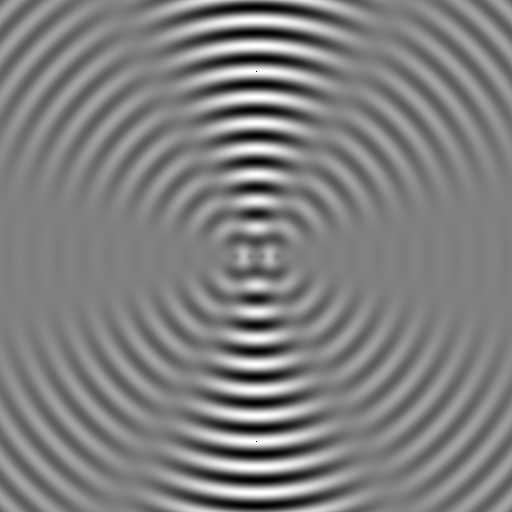
The best way to inspect the sound output is to use an oscilloscope that I luckily had bought for Arduino projects (mine is a Siglent SDS 1202X-E). This was the perfect solution to this data inspection problem; just hook it up to a 3.5 mm plug coming out of my phone, play the string, and watch the oscilloscope screen.

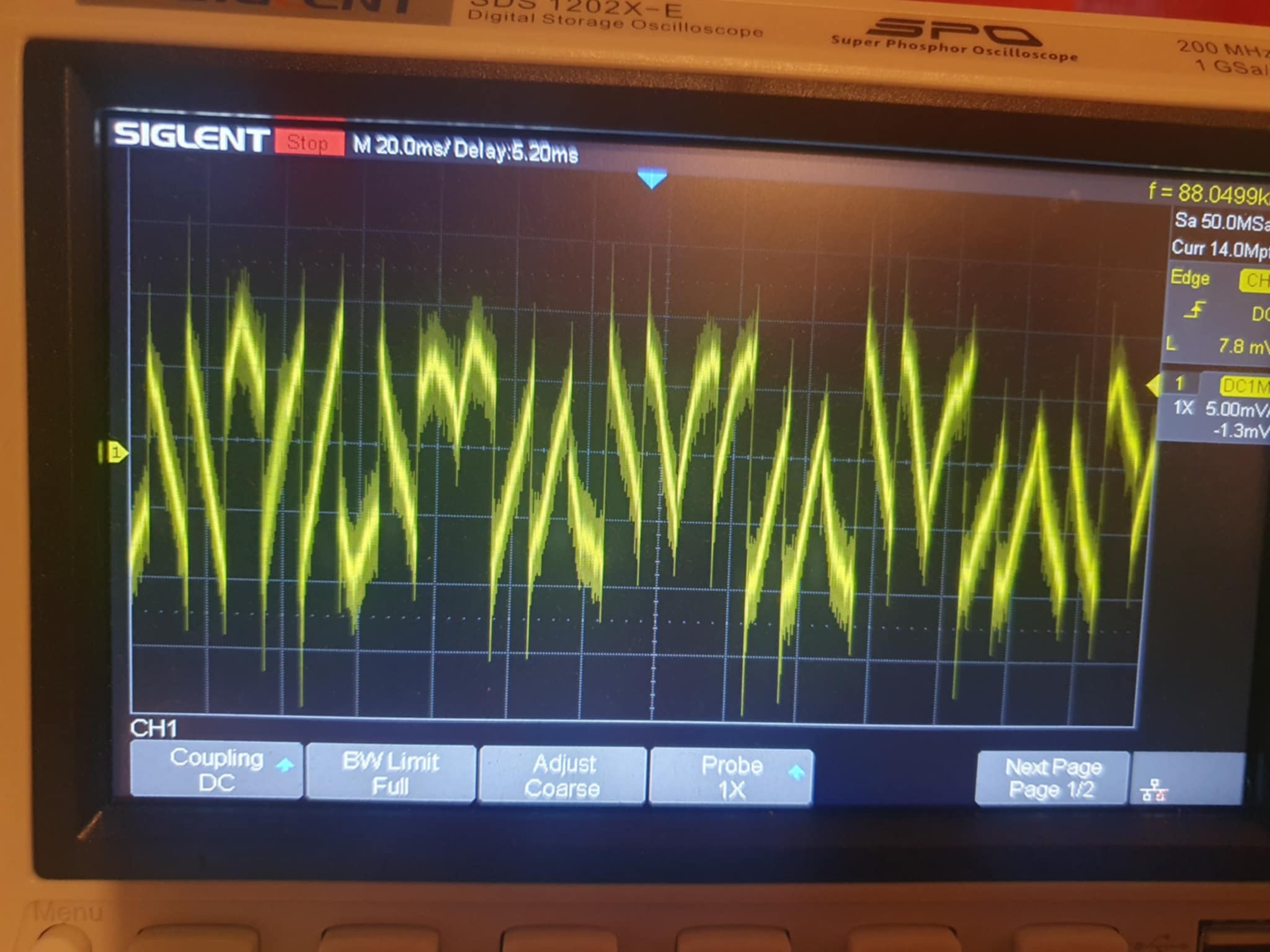
This particular example shows a buffer that updates too slow, such that the audio callback mostly receives repeated chunks of data. This I could never have learned without the oscilloscope.

I realized that perhaps I needed to use a ring buffer, a type of buffer with periodic boundary conditions, i.e. like a snake biting its own tail. In this type of buffer, there is a ‘write head’, and a ‘read head’. When the write head reaches the size of the buffer, it will continue overwriting the oldest data. The read head just runs after it, it should be slow enough so as not to overtake the write head, but fast enough that it wil not be overtaken by the write head. I borrowed a ring buffer class from Embedded Artistry, which contains all the details on how to read and write to such a buffer, as well as methods to measure the distance between the write and the read head. You can then instantiate the ringbuffer in the following way:

CircularBuffer<float> ringbuff = CircularBuffer<float>(BUFFER_SIZE);

After this, you can write data with a ‘put’ command:

ringbuff.put(Amplitude);

and read data with a get() command:

ringbuff.get()

Very convenient! That was it for the majority of the program, I will stop here since I covered the most important aspects, and the blog post is very long. I hope you learned something. See you later!

As you can see, these are hand-drawn sprite images for animating the main character of a game. I used the following method, which is perhaps best described as ‘reverse rotoscoping’: I downloaded a 3D character that performed a walking animation, then laid a paper on my screen, and traced the model with a pencil from different angles, and at different stages of the walk cycle. It’s important here to keep the center of the animation at a constant position throughout the cycle.

The perspectives were from south, south-east, east etc, totalling eight different perspectives. However, three of these can be generated by mirroring the opposite direction (east-west), reducing the total amount of drawn perspectives to five. Every walk cycle was cut up in five stages, such that adds up to 25 drawings. One can then scan these images, and cut them out (I used Inkscape for that).

I then used Unity to create an Android app with this animation, using the drawing as the main character. A ‘sprite renderer’ is necessary to add to the object that represents the player. I find the ‘animator’ in Unity a little bit confusing for creating animation, so I wrote my own code to swap sprites over time. In short, this comes down to defining a sprite list for every direction:

public List<Sprite> spriteMove = new List<Sprite>();

where the list can be loaded with sprites from the Unity UI, you simply drag and drop. Then, in order to cycle through the animations with a certain speed, I learned that it best to use the IEnumerator(), which is a function that runs coroutines. This function allows for breaks with a certain time extend, giving the choppy animation that I was looking for (Update() loop does not allow for breaks).

private void Start()
{
    StartCoroutine(PlayAnim());
}

IEnumerator PlayAnim()
{
    while (true) { 
        yield result new WaitForSeconds(0.25);
        spriteIndex++;
        spriteRenderer.sprite = spriteMove[spriteIndex];
    }
}

This serves as a simple example, of course one has to take care that the sprite index resets after a certain amount, and to implement the different perspectives using different sprite lists. I used a gargantuan conditional to assign eight joystick direction to eight animation perspectives. But everyone should find their own ways to do it. There is some more coding involved in camera movement and character movement, and a little modelling of the surroundings, but this is beyond the scope of this blog. The result of this project was fulfilling, and the hand drawnness of the character indeed gives it a somewhat artistic edge.

From what I understand, a phased array is basically a collection of regularly spaced oscillators that emit in the outward direction, each oscillator producing a wave with a spherical symmetry. The idea is that, due to interference, the array produces a (somewhat focused) beam of waves. The more oscillators, the more focused the beam becomes. These beams can be steered by subtle tuning of the phase difference between the individual oscillators. If all oscillators are oscillating in unison, the resulting beam will propagate perpendicular to the array.

This phenomenon is used for a range of tech applications, such as antenna’s (electromagnetic waves), and ultrasound imaging (ultrasonic acoustic waves). I was a bit inspired by this phenomenon, and formulated a vague goal for myself: to build a 2D phased array, for scanning 3D objects. The oscillators in question will be transducers that produce ultrasonic waves of 40 KHz, and should be individually controlled through a microcontroller. The amount of oscillators I have in mind is a 4x4 or 5x5 grid, the amount being limited by the amount of outputs on the microcontroller.

As a first step, I thought it would be a good idea to simulate these systems on a computer, to get a feeling for the behaviour of phased arrays. I started out with a script in Python that can simulate a 1D array of oscillators, it can be found here. Essentially, it’s just a superposition of circular waves,

\(// \psi(x,y)=e^{ikr}\),

for a spatial grid of 512 by 512 pixels.

I tried a row of 4 oscillators:

then steered it by changing the relative phases:

and extended it to 6 oscillators. It can be seen that the beam is more narrow:

and here is the power of the beam:

I did not take any attentuation of the waves into account, since I was just interested in the directionality.

Of course, I wanted to take it to the next level by extending these simulations to the third dimension, in order to investigate two dimensional arrays of oscillators. Since this is a bit heavy for Python (4 nested for-loops, need I say mo’), I turned to my favorite language, Julia. I wrote an object oriented script that treats the simulation like an object, and utilized the GPU for the heavy lifting, using the CUDA library. All of this was done in a handy Jupyter Notebook format. Just create a simulation using sim = SimulationWorld(…), and run it by run(sim), and the total psi(x,y,z) is outputted (is outputted a word?). This way, a grid of 512 x 512 x 1024 voxels (a quarter billion points), for 25 oscillators is simulated in 5 seconds on a laptop RTX 2060 graphics card.

Let’s focus on a simulation of 25 oscillators, i.e. a 5 by 5 grid. The spacing between the oscillators is half a wavelength. We can then take slices through the middle of psi(x,y,z) block to inspect the beam (the emitters are on the left side):

We can also inspect the power of the beam over this slice:

The nice thing about full 3D instead of 2D simulations is, besides the increased accuracy, the possibility of 3D visualisation. Let’s make beautiful 3D images of the beam making its way through space. One way to do this is by 3D voxel plotting, but this will burn your graphics card for the size of grid that we are interested in. Instead, it would be good to wrap isosurfaces of equal pressure/amplitude around the different regions in space. For this, we first have to find a suitable threshold for the amplitude, both positive and negative, and group connected regions together. Then, we wrap isosurfaces around these regions using a marching cubes algorithm (it’s part of a Julia package), which results in meshes for both positive and negative regions. Now, we can save these meshes into .obj files, and import them in Blender. I have to admit that in this last section I relied quite heavily on ‘vibe coding’, but whatever works works, and the result is quite amazing.

Here are waves emitted from the 25 oscillators, with a oscillator spacing of 0.5 wavelengths:

It can be seen that this leads to a nice, focused cone, with only small lobes on the sides. What happens when we increase the distance between the oscillators to a full wavelength?

It can be seen that significant side lobes exist, that carry a large portion of the total energy. The main beam also lost it’s circular shape, and instead has a more square-like outline. This seems like a good platform for studying the behaviour of the phased array. The next step is the experimental realization of such an array, I hope this will turn out good too. Stay tuned people.

I write about projects that I did. I do this to have some overview of what I do, plus I want to show things to people.

Here’s what I plan to write about:

• simulations
• microcontroller projects (often sound related)
• half finished games that I made (often mobile stuff)

Thanks,

Sam